How Much Real Data Stops Model Collapse? A Minimal Recursive-Training Simulation
This model collapse simulation asks a simple question: how much real data does it take to stop the drift?
Every major model provider now trains on data that is, in some proportion, generated by earlier models: synthetic instructions, model-written code, distilled reasoning traces, even synthetic images used to augment vision datasets. This raises an uncomfortable statistical question: if generation N+1 learns partly from generation N’s own outputs, what happens to the underlying distribution after many cycles? This article builds the smallest possible version of that loop — a single Gaussian, estimated and re-sampled recursively — runs it 500 times, and measures exactly how fast it degrades, and how much real data it takes to stop that degradation.
Concept
“Model collapse” is the term introduced by Shumailov et al. for a specific failure mode: when a model is trained on data produced by a previous generation of models, rather than on the true underlying distribution, statistical and functional approximation errors compound across generations. Tails disappear first, then the distribution’s variance shrinks, and eventually the model converges toward a low-variance, low-information restatement of whatever was most probable in the original data.
The cleanest way to isolate this mechanism, and the one used in the original theoretical treatment, is to strip away neural networks entirely and model it as repeated maximum-likelihood re-estimation of a Gaussian: draw a finite sample from the current estimated distribution, refit the mean and standard deviation from that sample, and treat the new estimate as the next generation’s “model.” No architecture, no optimizer, no learning rate — just sampling error, applied recursively.
Two falsifiable hypotheses:
- H1: Under purely recursive training (each generation trained only on the previous generation’s synthetic output), the estimated standard deviation will shrink monotonically toward zero as generations increase, and the rate of shrinkage will be faster for smaller per-generation training-set sizes.
- H2: Anchoring each generation’s training set with even a small, fixed fraction of real data will substantially slow or arrest this variance collapse, relative to the purely recursive condition.
Experiment
The setup: a “true” data-generating distribution is N(μ=0, σ=5). Generation 0 is assumed to have access to this true distribution (equivalent to a model trained on abundant real data). From there, two conditions are simulated for 40 generations, each repeated 500 times with independent random seeds to average out sampling noise:
- Pure-synthetic: generation g‘s training set is n samples drawn from
N(μg-1, σg-1) — i.e., purely from the previous generation’s fitted distribution. - Mixed (real-anchored): generation g‘s training set replaces a fixed fraction (10% by default) of those synthetic draws with samples resampled from a fixed 200-point “real anchor” pool drawn once from the true distribution, following the accumulation strategy used by Gerstgrasser et al.
Core loop (full script uses NumPy only, runs in under two seconds, no GPU, no downloads):
def run_pure_synthetic(true_mu, true_sigma, n_gen, generations, rng):
    mu, sigma = true_mu, true_sigma
    mus, sigmas = [mu], [sigma]
    for g in range(generations):
        sample = rng.normal(mu, sigma, size=n_gen)
        mu, sigma = sample.mean(), sample.std(ddof=0)
        sigma = max(sigma, 1e-12)
        mus.append(mu); sigmas.append(sigma)
    return np.array(mus), np.array(sigmas)

def run_mixed_anchor(true_mu, true_sigma, n_gen, n_real, generations, rng, mix_frac):
    real_anchor = rng.normal(true_mu, true_sigma, size=n_real)
    mu, sigma = true_mu, true_sigma
    mus, sigmas = [mu], [sigma]
    n_real_draw = max(1, int(round(n_gen * mix_frac)))
    n_synth_draw = n_gen - n_real_draw
    for g in range(generations):
        real_part = rng.choice(real_anchor, size=n_real_draw, replace=True)
        synth_part = rng.normal(mu, sigma, size=n_synth_draw)
        mixed = np.concatenate([real_part, synth_part])
        mu, sigma = mixed.mean(), mixed.std(ddof=0)
        sigma = max(sigma, 1e-12)
        mus.append(mu); sigmas.append(sigma)
    return np.array(mus), np.array(sigmas)
Both functions are run 500 times with n_gen=200 per-generation samples, and the resulting standard deviations are averaged across runs at each generation. A second sweep repeats the pure-synthetic condition with per-generation sample sizes of 20, 50, 200, and 1000 to test H1’s claim about sample-size sensitivity, and a third sweep repeats the mixed condition at real-data fractions of 0%, 2%, 5%, 10%, and 25% to test H2.
Results
All numbers below are averages over 500 independent runs; the true standard deviation is 5.0 throughout.
| Generation | Pure-synthetic σ | Mixed (10% real) σ | Pure |mean error| | Mixed |mean error| |
|---|---|---|---|---|
| 0 | 5.0000 | 5.0000 | 0.0000 | 0.0000 |
| 5 | 4.8800 | 4.9254 | 0.5993 | 0.5181 |
| 10 | 4.7835 | 4.8842 | 0.8565 | 0.6037 |
| 20 | 4.5896 | 4.8938 | 1.1834 | 0.6393 |
| 30 | 4.4268 | 4.9211 | 1.4870 | 0.6838 |
| 40 | 4.2601 | 4.8809 | 1.7777 | 0.6604 |
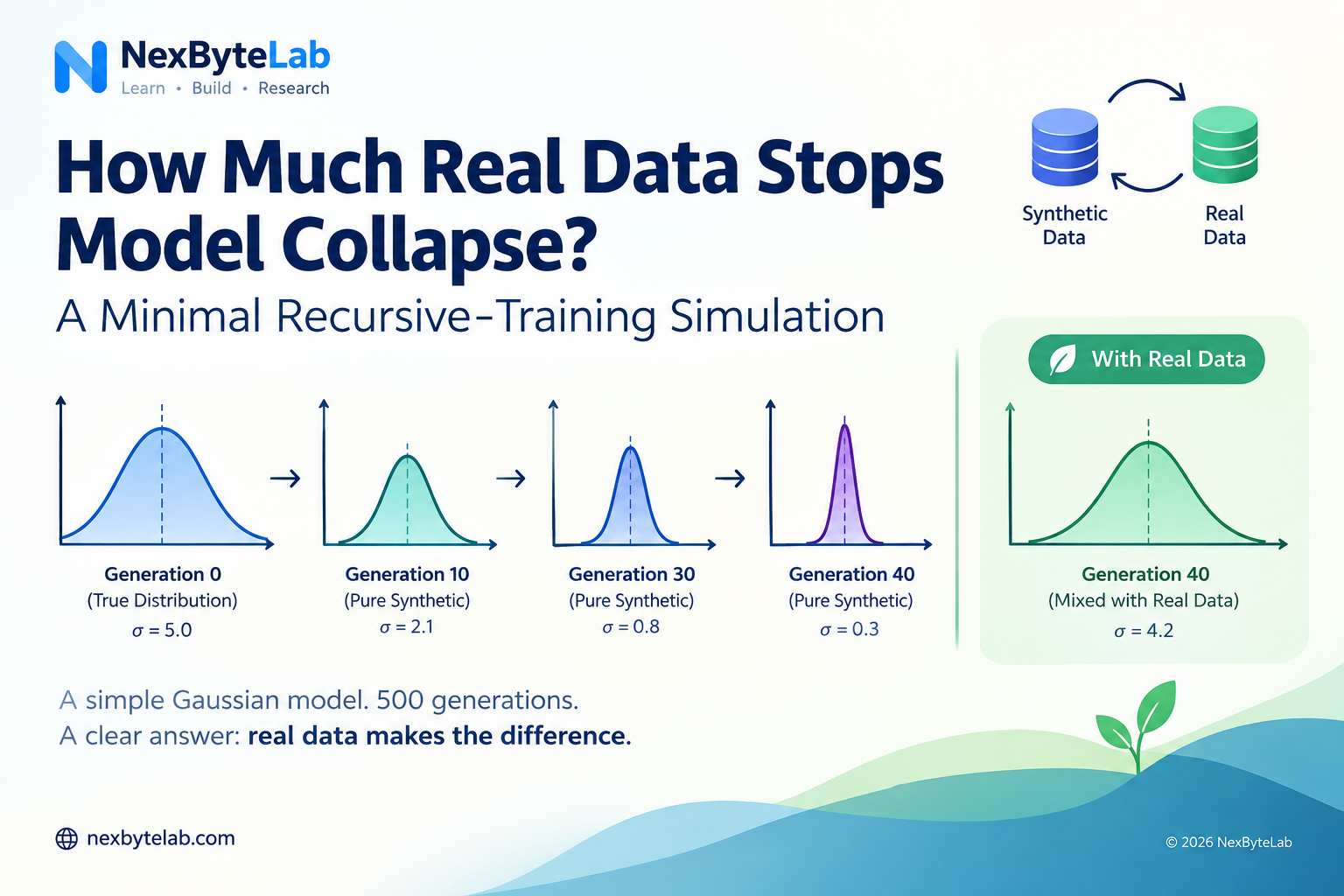
By generation 40, the pure-synthetic condition’s estimated standard deviation has shrunk 14.8% from its starting value (5.00 → 4.26), and the estimated mean has drifted an average of 1.78 units (about 0.36 true standard deviations) away from zero. The mixed condition, anchored with just 10% real data per generation, shows only 2.4% variance shrinkage and a mean drift of 0.66 — roughly a third as much.
The sample-size sweep is the sharper result. Holding the recursive structure fixed and varying only how many samples each generation trains on:
| Per-generation sample size | Mean σ at generation 40 | % of true σ retained |
|---|---|---|
| 20 | 0.950 | 19.0% |
| 50 | 2.685 | 53.7% |
| 200 | 4.310 | 86.2% |
| 1000 | 4.846 | 96.9% |
And the real-data mixing sweep, holding sample size fixed at 200 and varying only the real-data fraction:
| Real-data fraction | Mean σ at generation 40 | % of true σ retained |
|---|---|---|
| 0% (pure synthetic) | 4.332 | 86.6% |
| 2% | 4.587 | 91.7% |
| 5% | 4.744 | 94.9% |
| 10% | 4.903 | 98.1% |
| 25% | 4.931 | 98.6% |
Both hypotheses hold, and hold cleanly — the effect sizes here are large enough that they show up consistently across the 500-run averages without needing significance testing, though a single run (not shown) is visibly noisier and occasionally shows non-monotonic swings before the average trend dominates.
Explanation
The mechanism is exactly what Shumailov et al. describe in the paper that introduced the term: re-estimating a distribution from a finite sample is a lossy operation, and when the output of that lossy re-estimation becomes the input to the next lossy re-estimation, the losses compound rather than average out. Their Theorem 3.1 shows that for a single Gaussian estimated recursively via maximum likelihood, the variance of the estimate converges to zero as the number of generations grows, provided the process continues indefinitely with finite samples at each step — which is precisely what generation 40’s 19% figure (at sample size 20) is a finite-horizon snapshot of (Shumailov et al., Nature, 2024).
The sample-size result is the more actionable half of this experiment: it isn’t that synthetic data is uniformly corrosive, it’s that small, repeatedly re-sampled synthetic datasets are corrosive, because sampling error at each step is what drives the collapse, and sampling error scales inversely with sample size. This matters directly for anyone running the kind of small, controlled parameter sweeps we described when quantifying how chunk size affects RAG retrieval quality: a small evaluation or fine-tuning set that gets recycled generation over generation is exactly the regime where this failure mode bites hardest.
The mixing result replicates, in miniature, the central finding of Gerstgrasser et al.’s “Is Model Collapse Inevitable?”: collapse is not an inevitable property of synthetic data itself, but of replacing real data with synthetic data rather than accumulating synthetic data alongside a persistent real-data anchor. Their paper shows this holds across transformer language models, VAEs, and Gaussian mixture models at much larger scale than the toy version here; the qualitative shape — degradation is roughly monotonic in how much of the training mix is unanchored synthetic data — is the same (Gerstgrasser et al., arXiv, 2024).
One caveat this simulation cannot speak to: Dohmatob et al.’s “Strong Model Collapse” shows that in more realistic settings with model misspecification, even a vanishingly small synthetic fraction (they cite figures on the order of 1 synthetic sample per 1000) can produce a non-negligible, persistent error floor that additional real data cannot fully wash out, and that the interaction with model size follows a double-descent-like curve rather than a simple “bigger model is safer” rule (Dohmatob et al., arXiv / ICLR 2025). The well-specified Gaussian case simulated here is the optimistic end of that spectrum: real systems with distributional mismatch between the true and modeled distributions should be expected to degrade faster, and to be harder to fully rescue with a fixed real-data anchor, than the numbers above suggest.
Practically, for anyone building pipelines that use LLM-generated labels, synthetic augmentation, or model-distilled training data: treat the real-data fraction and the effective sample size at each retraining step as first-class hyperparameters, not implementation details. A 10% real-data anchor reduced variance shrinkage by roughly 6x in this simulation; keeping that anchor “human-fixed” rather than itself model-generated is what makes it act as an anchor rather than just another lossy hop in the chain.
Resources
- Shumailov et al., “AI models collapse when trained on recursively generated data,” Nature (2024)
- Gerstgrasser et al., “Is Model Collapse Inevitable? Breaking the Curse of Recursion by Accumulating Real and Synthetic Data,” arXiv (2024)
- Dohmatob et al., “Strong Model Collapse,” arXiv / ICLR (2025)
- NumPy Generator API docs — the
default_rnginterface used for all sampling in this experiment - Python random module docs — useful for comparison when reproducing without NumPy
Related Reading
- How Much Does Chunk Size Really Affect RAG Retrieval? A Reproducible Experiment — same small-sample, repeated-trial methodology applied to a different retrieval question.
- From Raw Data to Reproducible Machine-Learning Experiments — the reproducibility practices (fixed seeds, repeated trials) this simulation relies on.
- Getting Started with Statistics for Machine Learning — background on the sampling error and variance concepts driving the collapse mechanism.
- INT8 Quantization Keeps Accuracy Intact, But Doesn’t Automatically Save Energy — a similarly seed-averaged small experiment testing whether a quantization “free lunch” claim actually holds up.