Reproducing Double Descent: Why 300 Features Beat 39 on the Same 40 Data Points
There’s a piece of machine-learning folklore that gets repeated so often it starts to sound like a law of nature: more parameters relative to your data means more overfitting, and overfitting means worse test performance. It’s the textbook U-shaped bias-variance curve. It’s also, in a very specific and reproducible sense, wrong — and you don’t need a neural network or a GPU to see it break.
Concept
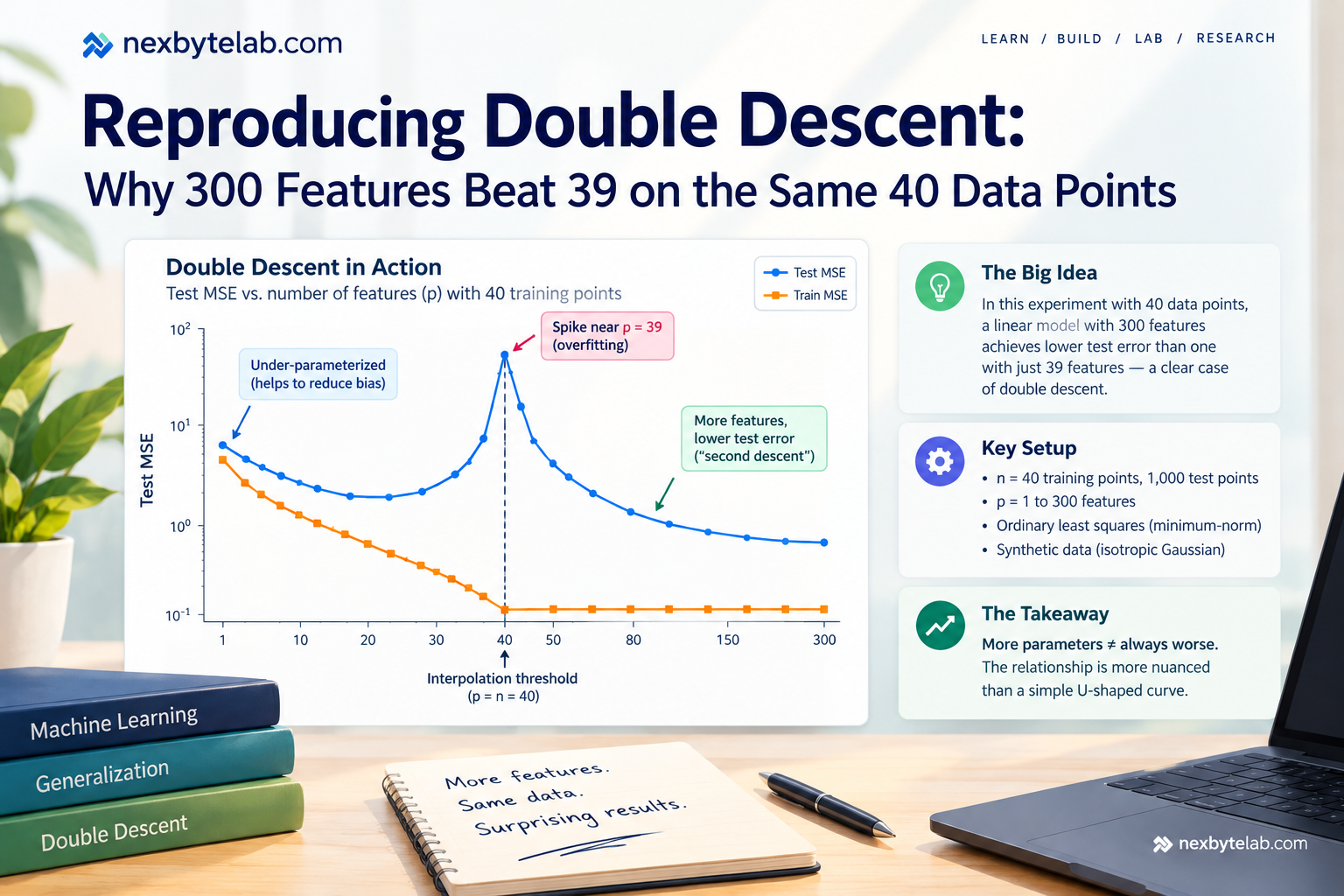
The phenomenon is called double descent. As you increase a model’s capacity while holding the training set fixed, test error first behaves the way classical statistics predicts: it falls, bottoms out, then rises as the model starts to overfit. But if you keep adding capacity past the point where the model can just barely fit (interpolate) every training point exactly — the interpolation threshold, where the number of parameters p equals the number of training points n — something unexpected happens. Test error, having spiked near that threshold, starts falling again. Keep adding parameters, and it can end up lower than anything achieved in the classical, safely under-parameterized regime.
This was first documented rigorously by Belkin et al. in 2019 and by Nakkiran et al.’s “Deep Double Descent,” and it’s since been shown to be a general property of interpolating estimators, not a deep-learning-specific quirk — it shows up in plain linear regression too.
Hypothesis (falsifiable): for a fixed, small training set (n = 40), sweeping the number of features p used by a minimum-norm ordinary-least-squares model from 1 up to 300 will not produce a monotonic or single-U-shaped test error curve. Test error will spike sharply as p approaches n, then decline again for p > n, eventually beating the best under-parameterized (p < n) model. If instead error simply falls or plateaus with no post-threshold recovery, the hypothesis is falsified.
Experiment
The setup deliberately avoids anything that could hide behind “the neural network learned something magic.” It’s ordinary least squares, fit with the Moore-Penrose pseudoinverse so the same solver works whether the system is under- or over-determined:
- Ground truth: a fixed random direction
beta_truein a 300-dimensional feature space. - Data: n = 40 training points and 1,000 held-out test points, each x drawn i.i.d. from an isotropic Gaussian in that 300-dim space, with y = x·beta_true + noise (noise std = 0.5).
- Model family: for each capacity p, use only the first p coordinates of x as features, and fit with the minimum-norm least-squares solution.
- Sweep: p from 1 to 300, densely sampled around p = n = 40 where the interesting behavior happens.
Key code (full script uses NumPy only, no scikit-learn, no GPU — runs in well under a second):
D, N_TRAIN, N_TEST, NOISE_STD, SEED = 300, 40, 1000, 0.5, 42
rng = np.random.default_rng(SEED)
beta_true = rng.normal(0, 1.0, size=D) / np.sqrt(D)

def make_data(n, rng_local):
    X = rng_local.normal(0, 1.0, size=(n, D))
    y = X @ beta_true + rng_local.normal(0, NOISE_STD, size=n)
    return X, y

X_train_full, y_train = make_data(N_TRAIN, rng)
X_test_full, y_test = make_data(N_TEST, rng)

def min_norm_ols(X, y):
    w, *_ = np.linalg.lstsq(X, y, rcond=None)   # minimum-norm solution
    return w

for p in p_values:
    Xtr, Xte = X_train_full[:, :p], X_test_full[:, :p]
    w = min_norm_ols(Xtr, y_train)
    train_mse.append(np.mean((Xtr @ w - y_train) ** 2))
    test_mse.append(np.mean((Xte @ w - y_test) ** 2))
Results
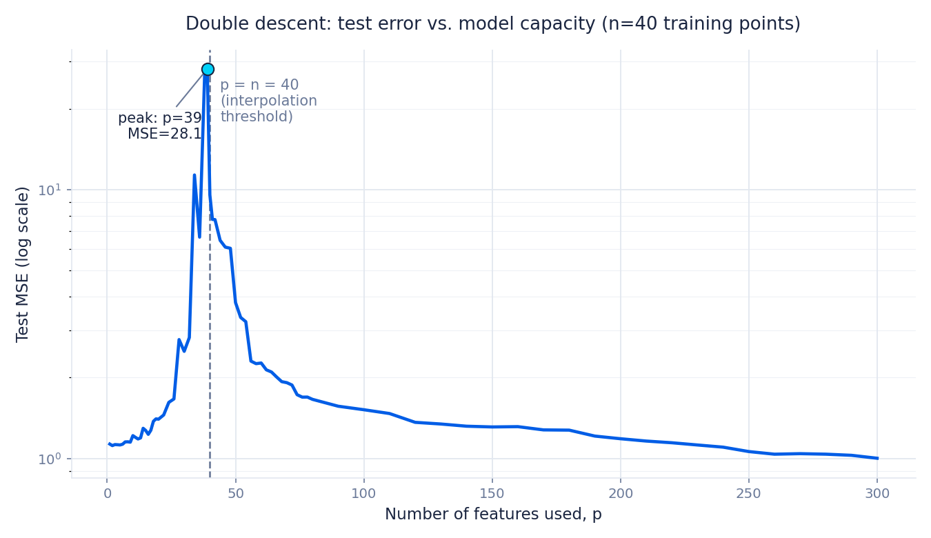
This is the actual output of the run above (seed = 42, single run — see the honesty note below).
| p (features) | p / n | Train MSE | Test MSE |
|---|---|---|---|
| 2 | 0.05 | 0.862 | 1.117 |
| 20 | 0.50 | 0.519 | 1.401 |
| 36 | 0.90 | 0.027 | 6.661 |
| 39 | 0.97 | 0.017 | 28.144 (peak) |
| 40 | 1.00 | 0.000 | 9.558 |
| 44 | 1.10 | 0.000 | 6.481 |
| 80 | 2.00 | 0.000 | 1.660 |
| 150 | 3.75 | 0.000 | 1.311 |
| 300 | 7.50 | 0.000 | 1.002 |
The numbers say exactly what the hypothesis predicted: test MSE climbs from 1.12 (at p = 2) up to a peak of 28.14 at p = 39 — one feature short of the interpolation threshold — a 25x spike over the best small model tested. Cross the threshold at p = 40 (where training error hits exactly 0.000, i.e. perfect interpolation of noisy data) and test MSE immediately drops to 9.56, then keeps falling smoothly as p grows. By p = 300, test MSE is 1.002 — not just recovered, but slightly better than the best under-parameterized model found anywhere in the sweep (1.117 at p = 2).
Honesty note: this is one run with one fixed seed. The overall shape (rise into a spike near p = n, then sustained decline) is a well-established analytical result for this exact linear/isotropic-Gaussian setup and is highly reproducible across seeds, but the precise peak height (28.14x) is somewhat seed- and noise-dependent — near p = n the design matrix is close to singular, so test error there can vary a great deal run to run. Anyone can verify this by changing SEED and rerunning; the spike moves around in magnitude but not in location.
Explanation
Why does this happen? The intuitive story: near p = n, the least-squares fit has just enough parameters to match the training data exactly, including its noise, but no extra parameters to be selective about how it does so — the minimum-norm solution has to route all the noise-fitting through directions with very small signal, which blows up the coefficient norm and the resulting variance. Once p exceeds n, there’s enough slack in the parameter space that the minimum-norm solution can fit the noise using “cheap” directions while still recovering the true signal direction reasonably well — effectively, implicit regularization from the minimum-norm choice starts working in the model’s favor again.
This isn’t a curiosity confined to toy linear models. A March 2025 analysis from a NYU-affiliated researcher, covered by MarkTechPost, argues double descent and related “benign overfitting” behavior aren’t actually mysterious or deep-learning-specific: both ResNets and plain linear models show the same U-then-recovery pattern, and the behavior is consistent with older generalization frameworks (PAC-Bayes, effective dimensionality) once you stop assuming worst-case bounds are tight. A 2024 paper, “Unified View of Grokking, Double Descent and Emergent Abilities”, goes further and proposes that double descent, grokking, and sudden capability jumps in larger models are all the same underlying phenomenon: a competition between memorization circuits and generalization circuits, where which one “wins” depends on the ratio of model size to the amount of data available for a given task.
There’s also an important practical caveat, and it’s worth taking seriously rather than treating double descent as a free lunch. A 2025 paper studying the phenomenon in neural quantum states (Double Descent: When Do Neural Quantum States Generalize?) found that the “second descent” only kicks in once network size is much larger than the effective dimensionality of the problem — in their setting, “out of reach for problems of practical interest.” That mirrors a pattern we’ve seen on this site before: as we found when testing whether the law of large numbers always saves you, a statistical guarantee that holds asymptotically can be practically useless if the regime where it kicks in is far outside what you can actually run. Double descent is real and reproducible in 40 lines of NumPy — but whether the “more parameters helps” side of the curve is reachable for your actual model and dataset is a separate, harder question.
Resources
- Understanding Generalization in Deep Learning: Beyond the Mysteries — MarkTechPost, March 2025, on the “soft inductive biases” framework unifying double descent and benign overfitting.
- Unified View of Grokking, Double Descent and Emergent Abilities — arXiv, 2024, memorization-vs-generalization circuit competition framework.
- Double Descent: When Do Neural Quantum States Generalize? — arXiv, 2025, on how far the second descent can be out of practical reach.
- Belkin et al., “Reconciling modern machine-learning practice and the classical bias-variance trade-off” — PNAS, 2019, the foundational paper.
- Nakkiran et al., “Deep Double Descent: Where Bigger Models and More Data Hurt” — arXiv, 2019.
- NumPy
linalg.lstsqdocumentation — the minimum-norm solver used in this experiment.
Related Reading
- Honest Write-Up: The Law of Large Numbers Doesn’t Always Save You — another case where a textbook statistical guarantee breaks down outside its practical regime.
- How Much Real Data Stops Model Collapse? A Minimal Recursive-Training Simulation — same experimental-research approach applied to a different generalization failure mode.
- Getting Started with Statistics for Machine Learning — the bias-variance foundations that double descent complicates.