
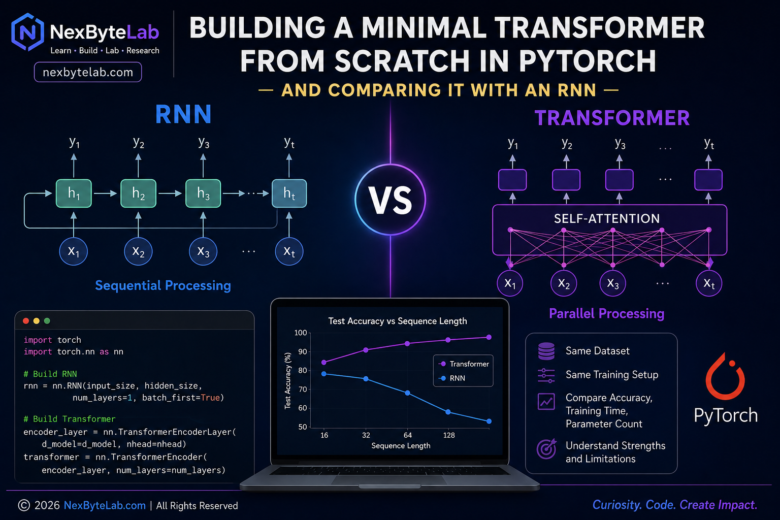
Building a Minimal Transformer From Scratch in PyTorch — and Comparing It With an RNN
This is a transformer from scratch in PyTorch build, compared directly against an RNN so the difference isn’t just theoretical.
In the previous article, we explored the idea behind Transformers: instead of processing a sequence strictly one element at a time, a Transformer uses self-attention to learn which parts of that sequence matter to one another.
But understanding an architecture on paper and observing its behaviour are two different things.
So this time, we are going to treat the question as a small experiment.
If we give a simple RNN and a small Transformer the same sequence-learning problem, what differences can we actually observe?
We will build both models in PyTorch, train them under controlled conditions, and compare their learning behaviour.
The objective is not to prove that “Transformers are better than RNNs.”
That would be far too broad a conclusion for one experiment.
Instead, the objective is to understand why their architectures behave differently.
1. The Research Question
Our experiment begins with a simple question:
How does a Transformer compare with a recurrent neural network when learning relationships across a sequence?
This question matters because RNNs and Transformers process sequences in fundamentally different ways.
A traditional RNN maintains a hidden state that evolves as it moves through the sequence. PyTorch describes its basic recurrence as:
hₜ = tanh(xₜWᵀᵢₕ + bᵢₕ + hₜ₋₁Wᵀₕₕ + bₕₕ)
In other words, the representation at time t depends partly on the representation from time t−1 [1].
A Transformer takes a different approach.
Vaswani and colleagues proposed an architecture that removed recurrence from its core and instead relied on attention mechanisms. This allows relationships between positions to be modelled more directly and allows much of the sequence computation to be parallelised during training [2].
Our experiment will make that architectural difference visible.
2. Our Hypothesis
Before running an experiment, it is good scientific practice to state what we expect.
Hypothesis
For a task requiring information from distant positions in a sequence:
A Transformer should be able to learn the dependency effectively because self-attention allows information at distant positions to interact directly. A simple RNN may find the same dependency harder as the sequence becomes longer because information is propagated recurrently through successive hidden states.
Notice the wording.
We are not saying:
“The Transformer will always beat the RNN.”
That would not be scientifically defensible.
Performance depends on the dataset, architecture, sequence length, parameter count, optimisation procedure, hardware, random initialization and many other factors.
Our hypothesis concerns this particular experiment.
3. Designing a Simple Experiment
Real-world language datasets introduce many variables:
- vocabulary size,
- tokenisation,
- ambiguous language,
- class imbalance,
- noisy labels,
- pretrained embeddings,
- and dataset-specific biases.
Those are important in real research, but they can make it difficult to understand why a model behaves differently.
So we will begin with a synthetic dataset.
This is common in scientific experimentation: simplify the environment so that the variable of interest becomes easier to observe.
4. The Task: Can the Model Remember a Distant Relationship?
Suppose we generate sequences such as:
3 8 1 4 7 2 9 6 5 3
The first number is 3.
The last number is also 3.
So the label is:
1
Now consider:
3 8 1 4 7 2 9 6 5 6
The first and last numbers are different.
The label becomes:
0
Our classification rule is therefore extremely simple:
Label = 1 if the first token equals the last token; otherwise Label = 0.
Why choose such an artificial task?
Because the relationship we care about is completely known.
The model cannot solve the problem reliably merely by understanding an individual token. It needs information about two different positions in the sequence.
More importantly, we can increase the distance between those positions simply by increasing the sequence length.
That gives us a small laboratory for studying sequence dependency.
5. Experimental Controls
If we want a meaningful comparison, we should avoid changing many things at once.
We therefore keep the following conditions as similar as practical:
| Variable | Setting |
|---|---|
| Task | Binary sequence classification |
| Vocabulary | Digits 0–9 |
| Training samples | 6,000 |
| Test samples | 2,000 |
| Sequence length | 64 |
| Embedding dimension | 64 |
| Optimizer | Adam |
| Learning rate | 0.002 |
| Batch size | 128 |
| Loss function | Cross-entropy |
| Random seed | 42 |
There is an important caveat.
Even when embedding sizes and training data are identical, an RNN and a Transformer do not necessarily contain the same number of trainable parameters.
Therefore, we should report parameter counts rather than casually calling the experiment “perfectly fair.”
This distinction matters in serious model comparison.
6. Step One: Make the Experiment Reproducible
Machine-learning experiments contain randomness.
Weights are randomly initialized. Training samples may be shuffled. Some hardware operations can also introduce nondeterministic behaviour.
We therefore begin by fixing our random seeds.
import random
import time

import numpy as np
import torch
import torch.nn as nn
from torch.utils.data import DataLoader, TensorDataset

SEED = 42

random.seed(SEED)
np.random.seed(SEED)
torch.manual_seed(SEED)

if torch.cuda.is_available():
    torch.cuda.manual_seed_all(SEED)

device = torch.device(
    "cuda" if torch.cuda.is_available() else "cpu"
)

print("Device:", device)
Setting a seed does not magically guarantee identical results across every possible hardware and software configuration, but it removes an important source of experimental variation.
7. Step Two: Generate the Dataset
We now create the synthetic sequences.
VOCAB_SIZE = 10
SEQ_LEN = 64

TRAIN_SIZE = 6000
TEST_SIZE = 2000


def create_dataset(size, seed):

    generator = torch.Generator()
    generator.manual_seed(seed)

    X = torch.randint(
        0,
        VOCAB_SIZE,
        (size, SEQ_LEN),
        generator=generator
    )

    y = torch.randint(
        0,
        2,
        (size,),
        generator=generator
    )

    same = y == 1
    different = y == 0

    # Positive examples:
    # first token == last token
    X[same, -1] = X[same, 0]

    # Negative examples:
    # guarantee that last token differs
    # from the first
    offsets = torch.randint(
        1,
        VOCAB_SIZE,
        (different.sum(),),
        generator=generator
    )

    X[different, -1] = (
        X[different, 0] + offsets
    ) % VOCAB_SIZE

    return X, y


X_train, y_train = create_dataset(
    TRAIN_SIZE,
    seed=1
)

X_test, y_test = create_dataset(
    TEST_SIZE,
    seed=2
)
We deliberately construct approximately balanced positive and negative examples.
This prevents a model from achieving impressive-looking accuracy simply by repeatedly predicting the majority class.
8. Build the RNN Baseline
A baseline is extremely important in machine learning.
Without one, saying that a model achieves “90% accuracy” tells us surprisingly little.
Perhaps an extremely simple model achieves 91%.
Our first baseline is a basic Elman RNN.
class RNNClassifier(nn.Module):

    def __init__(
        self,
        vocab_size=10,
        embedding_dim=64,
        hidden_dim=64
    ):

        super().__init__()

        self.embedding = nn.Embedding(
            vocab_size,
            embedding_dim
        )

        self.rnn = nn.RNN(
            input_size=embedding_dim,
            hidden_size=hidden_dim,
            batch_first=True
        )

        self.classifier = nn.Linear(
            hidden_dim,
            2
        )

    def forward(self, x):

        x = self.embedding(x)

        output, hidden = self.rnn(x)

        final_hidden = hidden[-1]

        return self.classifier(final_hidden)
Conceptually, information moves through the RNN like this:
x1 → h1 → h2 → h3 → ... → h64
                         ↓
                    prediction
The final hidden state must contain enough information for the classifier to determine the answer.
PyTorch’s nn.RNN implements this recurrent hidden-state structure directly [1].
9. Build the Minimal Transformer
Now we build our Transformer classifier.
For educational clarity, we will use PyTorch’s TransformerEncoderLayer.
PyTorch describes this component as consisting of self-attention and a feed-forward network, based on the architecture introduced in Attention Is All You Need [3].
class TransformerClassifier(nn.Module):

    def __init__(
        self,
        vocab_size=10,
        seq_len=64,
        d_model=64,
        nhead=4,
        dim_feedforward=128,
        num_layers=2
    ):

        super().__init__()

        self.embedding = nn.Embedding(
            vocab_size,
            d_model
        )

        self.position = nn.Parameter(
            torch.randn(
                1,
                seq_len,
                d_model
            ) * 0.02
        )

        encoder_layer = nn.TransformerEncoderLayer(
            d_model=d_model,
            nhead=nhead,
            dim_feedforward=dim_feedforward,
            dropout=0.0,
            batch_first=True
        )

        self.encoder = nn.TransformerEncoder(
            encoder_layer,
            num_layers=num_layers
        )

        self.classifier = nn.Linear(
            d_model,
            2
        )

    def forward(self, x):

        x = self.embedding(x)

        x = x + self.position[:, :x.size(1)]

        x = self.encoder(x)

        final_token = x[:, -1]

        return self.classifier(final_token)
Notice something important.
The last token’s representation is processed through self-attention.
That means it can potentially obtain information directly from the first token rather than depending on information being propagated sequentially through every intermediate position.
Conceptually:
Token 1 ───────────────┐
Token 2 ────────────┐  │
Token 3 ─────────┐  │  │
...              │  │  │
Token 64 ←───────┴──┴──┘
        ↓
   prediction
This is not a literal diagram of every Transformer computation, but it illustrates the important architectural distinction.
10. Attention in One Equation
The central operation introduced by Vaswani et al. is scaled dot-product attention:
Attention(Q, K, V) = softmax(QKᵀ / √dₖ)V
[2]
In plain English:
- create a query representing what a token is looking for,
- compare it with keys representing other tokens,
- calculate attention scores,
- normalise those scores,
- combine the corresponding values.
For our task, the network has the opportunity to learn that information near the beginning of the sequence is useful when constructing the representation used for the final classification.
11. One Training Function for Both Models
Now comes an important experimental decision.
Both models should go through the same training procedure.
def train_model(
    model,
    train_loader,
    test_loader,
    epochs=8,
    learning_rate=0.002
):

    model = model.to(device)

    optimizer = torch.optim.Adam(
        model.parameters(),
        lr=learning_rate
    )

    criterion = nn.CrossEntropyLoss()

    history = []

    start_time = time.perf_counter()

    for epoch in range(epochs):

        model.train()

        total_loss = 0
        correct = 0
        total = 0

        for X_batch, y_batch in train_loader:

            X_batch = X_batch.to(device)
            y_batch = y_batch.to(device)

            optimizer.zero_grad()

            predictions = model(X_batch)

            loss = criterion(
                predictions,
                y_batch
            )

            loss.backward()
            optimizer.step()

            total_loss += (
                loss.item() *
                y_batch.size(0)
            )

            predicted_labels = (
                predictions.argmax(dim=1)
            )

            correct += (
                predicted_labels == y_batch
            ).sum().item()

            total += y_batch.size(0)

        train_accuracy = correct / total
        train_loss = total_loss / total

        # Evaluation

        model.eval()

        test_correct = 0
        test_total = 0

        with torch.no_grad():

            for X_batch, y_batch in test_loader:

                X_batch = X_batch.to(device)
                y_batch = y_batch.to(device)

                predictions = model(X_batch)

                predicted_labels = (
                    predictions.argmax(dim=1)
                )

                test_correct += (
                    predicted_labels == y_batch
                ).sum().item()

                test_total += y_batch.size(0)

        test_accuracy = (
            test_correct / test_total
        )

        history.append({
            "epoch": epoch + 1,
            "loss": train_loss,
            "train_accuracy": train_accuracy,
            "test_accuracy": test_accuracy
        })

        print(
            f"Epoch {epoch + 1:02d} | "
            f"Loss: {train_loss:.4f} | "
            f"Train Acc: {train_accuracy:.4f} | "
            f"Test Acc: {test_accuracy:.4f}"
        )

    elapsed = (
        time.perf_counter() - start_time
    )

    return model, history, elapsed
12. Prepare the DataLoaders
BATCH_SIZE = 128

train_dataset = TensorDataset(
    X_train,
    y_train
)

test_dataset = TensorDataset(
    X_test,
    y_test
)

train_loader = DataLoader(
    train_dataset,
    batch_size=BATCH_SIZE,
    shuffle=True
)

test_loader = DataLoader(
    test_dataset,
    batch_size=BATCH_SIZE
)
Both models now see the same training and test data.
13. Count the Parameters
Before comparing results, we should know the size of each model.
def count_parameters(model):

    return sum(
        p.numel()
        for p in model.parameters()
        if p.requires_grad
    )


rnn_model = RNNClassifier()

transformer_model = TransformerClassifier()

print(
    "RNN parameters:",
    count_parameters(rnn_model)
)

print(
    "Transformer parameters:",
    count_parameters(transformer_model)
)
This number should be included with the experimental results.
Why?
Because model capacity itself can influence performance.
A model with substantially more parameters may have an advantage unrelated to the architectural property we intended to study.
14. Run the RNN Experiment
torch.manual_seed(SEED)

rnn_model = RNNClassifier()

rnn_model, rnn_history, rnn_time = train_model(
    rnn_model,
    train_loader,
    test_loader
)

print(
    "RNN training time:",
    round(rnn_time, 2),
    "seconds"
)
Record the output.
Do not decide whether the RNN is “good” or “bad” yet.
We still need the comparison.
15. Run the Transformer Experiment
torch.manual_seed(SEED)

transformer_model = TransformerClassifier()

transformer_model, transformer_history, transformer_time = train_model(
    transformer_model,
    train_loader,
    test_loader
)

print(
    "Transformer training time:",
    round(transformer_time, 2),
    "seconds"
)
Now we have two sets of observations generated under broadly controlled conditions.
16. Record the Results — Don’t Invent Them
After running the experiment, fill in the following table using the actual output from your machine.
| Metric | RNN | Transformer |
|---|---|---|
| Trainable parameters | Run experiment | Run experiment |
| Final training loss | Run experiment | Run experiment |
| Final training accuracy | Run experiment | Run experiment |
| Final test accuracy | Run experiment | Run experiment |
| Training time | Run experiment | Run experiment |
Why leave the numbers blank in the published experimental template?
Because benchmark numbers should be measured, not imagined.
Training time in particular depends heavily on hardware, PyTorch version, CPU/GPU implementation and system configuration.
Once the experiment has been executed, those measured numbers can be reported together with the environment in which they were obtained.
17. What Should We Look For?
Accuracy alone is not enough.
There are at least four useful observations.
1. Learning speed
How quickly does training loss fall?
If one architecture reaches useful accuracy in fewer epochs, that tells us something about optimisation on this particular problem.
2. Generalisation
Compare training accuracy with test accuracy.
A model achieving:
Training accuracy: 99%
Test accuracy:     55%
has learned something very different from a model achieving:
Training accuracy: 95%
Test accuracy:     94%
The second model is generalising much better to unseen examples.
3. Computational time
Measure training time.
But interpret it carefully.
The original Transformer paper highlighted the architecture’s parallelisability [2]. That does not mean a tiny Transformer must always run faster than a tiny RNN on every CPU or GPU.
Hardware, batch size, sequence length and implementation all matter.
4. Parameter count
A model that wins with ten times as many parameters creates a different scientific conclusion from a similarly sized model that wins.
Always report model size.
18. The More Interesting Experiment: Increase Sequence Length
Our first experiment uses sequences of length 64.
Now change:
SEQ_LEN = 16
and repeat the experiment.
Then try:
SEQ_LEN = 32
followed by:
SEQ_LEN = 64
and perhaps:
SEQ_LEN = 128
Record the test accuracy for each model.
Your table becomes:
| Sequence Length | RNN Accuracy | Transformer Accuracy |
|---|---|---|
| 16 | measured | measured |
| 32 | measured | measured |
| 64 | measured | measured |
| 128 | measured | measured |
This is much more interesting scientifically.
We have now changed an independent variable:
sequence length
and observed a dependent variable:
model performance.
The question becomes:
What happens to each architecture as the dependency between relevant positions becomes increasingly distant?
Now we are conducting an experiment rather than simply running two pieces of code.
19. Why Might the Architectures Behave Differently?
Consider the RNN.
To connect information from the first position with the final prediction, the recurrent computation proceeds through many intermediate steps:
h1 → h2 → h3 → h4 → ... → h64
The RNN’s hidden state acts as a continually updated memory.
The Transformer creates a different computational structure.
Self-attention allows a representation at one position to interact with representations at other positions within an attention layer.
Vaswani et al. explicitly discussed this shorter path between long-range dependencies as one motivation for self-attention [2].
That does not guarantee better performance.
It changes the route through which information can travel.
And that is the architectural idea our experiment is designed to expose.
20. But There Is a Catch
At this point, it would be tempting to conclude:
“Transformers solve long sequences, therefore Transformers are always superior.”
That conclusion would be wrong.
Standard self-attention has its own computational cost.
For a sequence containing n tokens, the attention score matrix contains relationships between pairs of positions. Consequently, the computational and memory burden associated with standard attention grows roughly quadratically with sequence length.
Conceptually:
Sequence length = n

Attention relationships ≈ n × n
So increasing the context from 1,000 to 10,000 tokens is not computationally trivial.
This limitation has motivated extensive research into efficient attention and alternative long-context architectures.
Every architecture makes trade-offs.
21. What Does This Experiment Actually Prove?
Very little — and that is an important scientific lesson.
One synthetic experiment cannot prove that Transformers are universally better than RNNs.
Our results apply only to:
- this synthetic task,
- these architectures,
- these hyperparameters,
- this training procedure,
- these sequence lengths,
- and the software/hardware environment used.
A stronger study would repeat each experiment using multiple random seeds and report the mean and variation across runs.
It would also attempt to control parameter counts more closely.
A serious extension might compare:
RNN vs LSTM vs GRU vs Transformer
rather than using only a basic RNN.
Why?
Because LSTMs were specifically developed to address some of the difficulties recurrent networks experience in learning long-term dependencies.
Our basic RNN therefore represents a useful educational baseline, not the strongest possible recurrent architecture.
22. Turning a Tutorial Into a Research Experiment
This small example illustrates an important difference between learning machine learning and researching machine learning.
A tutorial asks:
How do I build a Transformer?
An experiment asks:
Under what conditions does the Transformer behave differently, and why?
That change in question forces us to think about:
- hypotheses,
- baselines,
- controls,
- metrics,
- reproducibility,
- confounding variables,
- limitations,
- and evidence.
Those habits matter far beyond Transformers.
They are at the heart of good experimental machine learning.
23. What We Learned
The RNN and Transformer approach the same sequence problem in fundamentally different ways.
An RNN repeatedly updates a hidden state:
previous state + current input → new state
A Transformer uses self-attention to model interactions between positions.
Neither mechanism should be declared universally superior based on a toy experiment.
Instead, our experiment gives us a controlled environment in which we can observe the consequences of those architectural choices.
That is a much more useful conclusion than simply saying:
“Transformers are better.”
24. The Bigger Lesson
Perhaps the most important result of this experiment has nothing to do with Transformers.
It is the methodology.
When someone claims:
“Model A is better than Model B,”
we should immediately ask:
Better at what?
Then:
On which dataset?
Using which metric?
With how many parameters?
Using what hyperparameters?
Across how many runs?
On what hardware?
And was everything else held reasonably constant?
Those questions separate a benchmark from a marketing claim.
The goal of machine-learning research is not merely to obtain a number.
It is to understand why we obtained it and under what conditions it remains true.
Next Experiment
Our experiment raises another question.
If a basic RNN struggles as dependencies become longer, recurrent neural networks already have architectures designed specifically to improve memory.
The obvious next comparison is therefore:
RNN vs LSTM vs GRU vs Transformer: Does Attention Really Win on Long Sequences?
This time, instead of testing a single sequence length, we can systematically vary it:
16 → 32 → 64 → 128 → 256
We can run each configuration multiple times, calculate mean accuracy and standard deviation, plot learning curves, compare parameter counts and measure training time.
At that point, we will no longer have just a coding tutorial.
We will have a small reproducible machine-learning study.
References
[1] PyTorch Documentation. torch.nn.RNN. PyTorch documentation. The documentation defines PyTorch’s implementation of a multi-layer Elman RNN and its recurrent hidden-state computation.
PyTorch RNN Documentation
[2] Vaswani, A., Shazeer, N., Parmar, N., et al. (2017). Attention Is All You Need. Advances in Neural Information Processing Systems (NeurIPS 2017). The paper introduced the Transformer architecture based on attention mechanisms without recurrence or convolution in its core architecture.
Original Transformer Paper — arXiv
[3] PyTorch Documentation. TransformerEncoderLayer. PyTorch’s reference implementation contains self-attention and feed-forward components and is based on the architecture introduced in Attention Is All You Need.
PyTorch TransformerEncoderLayer Documentation
[4] PyTorch Documentation. TransformerEncoder. PyTorch describes TransformerEncoder as a stack of Transformer encoder layers and notes that the implementation is intended as a reference implementation for foundational understanding.
PyTorch TransformerEncoder Documentation
Experiment reproducibility note:
The code in this article intentionally uses a synthetic dataset so that the experiment can be reproduced without downloading proprietary data or relying on external APIs. Reported benchmark results should only be added after executing the supplied experiment and recording the software version, hardware environment and random seeds used.
Related Reading
- Transformers Explained — the concept behind the architecture, explained first
- Papers Explained: Attention Is All You Need — the original paper this implementation is based on